Modeling Expert's Opinions...Making Models Less Stupid

April 07, 2024
by a searcher in Portland, OR, USA
It's common knowledge to factor in base case, worst case and best case scenarios in our models. We may, as a follow on analysis, do a sensitivity analysis, e.g., letting one factor change while leaving all other factors unchanged. The world doesn't really work that way. Let's take a step back -- and not deprive ourselves.
Are we properly representing the variability, or uncertainty, in any given factor in and of itself? Moreover, what's the likelihood of the base case, worst case and best case (or, to rephrase it, a middle, low or high value)? Is a base case occurring at 35% of the time meaningfully different (See Note 1) than that occurring at 65% of the time? Or, what about a worst case of 10% compared to a 1% chance? Or, say, what about a best case with 5% chance versus 15% chance of occurrence?
It's not just a matter of incrementally stepping through the values (See Note 2) of any given factor in your analysis. Without me showing you any proof of it, I'd say you would still be assuming a certain kind of underlying variability, or uncertainty, unknowingly and/or without stating it with each incremental step. Instead, a much better representation is to fit the values of your factor(s) to the best approximation(s) of probability distribution(s).
How can we do it? As an example, let's say you're interviewing an expert on base case, worst case and best case for a key factor known as equipment utilization (in days out per contract) for bucket trucks in a fleet. This could be research gathered either empirically, a.k.a., data, or qualitatively, a.k.a., opinions [See Note 3]. Each case would have a pairing, e.g., pair up each value with its corresponding probability. Since we're dealing with three cases, we would have at least three pairs.
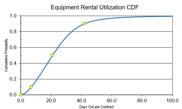
As an illustration, let's say our pairs, i.e., "days out per contract" by "percent of time", reflect the expert's opinions, as follows: (7 days or less, 10%) as worst; (21 days or less, 50%) as base; and (42 days or less, 90%) as best case. Next, I would run these pairs through a fitting algorithm [See Note 4]. As a result, we, now, have a much better representation and distribution for equipment utilization as probabilities of rental days out per contract.

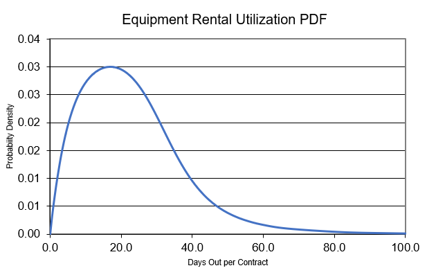
Remember, a contract is created when a customer rents our equipment. We're evaluating the contractual days our customers hire us between pickups and drop offs. Loosely speaking, we can think of the four dots above as also three opinions plus an undeniable fact that we can only have non-negative days out per contract. Below, we see that our expert's opinions don't follow a symmetric distribution; rather, it has skewness.

We have a much better story [See Note 5]: we can better say what we expect for equipment rental utilizations of our bucket trucks. We can better reflect our expert's opinions as probability weighted outcomes. Assigning the appropriate level of confidence, we can state -- then, if asked -- the range of values to express our pessimism/optimism [See Note 6] in our bucket truck analogy. As a teaser, we could begin to make better statements about revenue, EBITDA or free cashflow projections over low/high probability events, including tail-end events given our bucket trucks and other factors, variables or levers -- and so much more with the right level of confidence [See Note 7]. Referencing the right tail, we can see that making a bet on 60 or more days out per contract is fast approaching the realm of impossibilities without further interventions, optimizations, improvements and/or innovations. In closing, better understand and incorporate the underlying process that governs each factor, variable, or lever, as shown in this post, and make less wrong, less stupid models.
Note 1: I used "meaningfully different" rather than "statistically different" to avoid any misleading notions.
Note 2: Values having an equal chance happening are best described as coming from an uniform distribution.
Note 3: I'm posing the problem as having an absence of real data to fit -- and that we only have three estimated quantiles through an interview research technique (not covered).
Note 4: This is the Metalog function that converts our expert's opinions to continuous probability distributions that can be used in simulations.
Note 5: There are several ways, which are not covered here, to further incorporate these simulated results into our analysis.
Note 6: To say it even less elegantly, it may be a good way to call out #$@&%*!? if you find that someone else is not in touch with reality, assuming we've locked in our expert's opinions well enough.
Note 7: This post is one step used to build Monte Carlo simulations (not covered) that provide a look into thousands to millions of many small experiments by simultaneously changing many variables given more realistic weights.